intro_timeseriesdatasets

library(timeSeriesDataSets)

library(ggplot2)

Introduction

The timeSeriesDataSets package provides a collection of time series datasets for R, with suffixes (_ts, _mts, _tbl_ts) added based on the object type and class to clearly indicate their time series nature. This helps users easily identify time series datasets by their names. The datasets are sourced from various R packages, with modified names to reflect their time series structure. In this vignette, we will explore these datasets and demonstrate how to use them in your analyses.

Getting Started

To use the datasets from the timeSeriesDataSets package, you first need to install and load the package. You can install it from CRAN or from a local source if you’re developing it.

# Install the package from CRAN
# install.packages("timeSeriesDataSets")

# Load the package
library(timeSeriesDataSets)

Datasets Overview

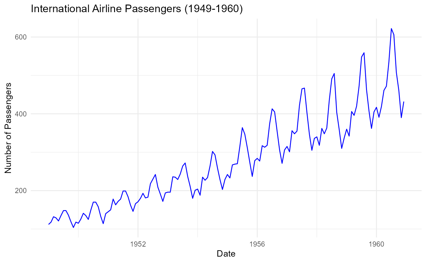
The AirPassengers_ts dataset is a classic time series that shows the monthly number of passengers from 1949 to 1960. Note that the timeSeriesDataSets package adds a _ts suffix to identify datasets like AirPassengers_ts as time series.

# Load the dataset
data("AirPassengers_ts")

# Check the class of the dataset
class(AirPassengers_ts)
#> [1] "ts"

# Display the first few rows of the dataset
head(AirPassengers_ts)
#> [1] 112 118 132 129 121 135

Time Series Visualization

You can use these time series datasets for various time series analyses and visualizations. For example, you can plot the data to visualize trends over time.

# Convert AirPassengers to a data frame for use with ggplot2
air_df <- data.frame(
  Month = time(AirPassengers_ts),
  Passengers = as.numeric(AirPassengers_ts)
)

# Time series plot
ggplot(air_df, aes(x = Month, y = Passengers)) +
  geom_line(color = "blue") +
  labs(title = "International Airline Passengers (1949-1960)",
       x = "Date", y = "Number of Passengers") +
  theme_minimal()
#> Don't know how to automatically pick scale for object of type <ts>. Defaulting
#> to continuous.

Trend and Seasonality

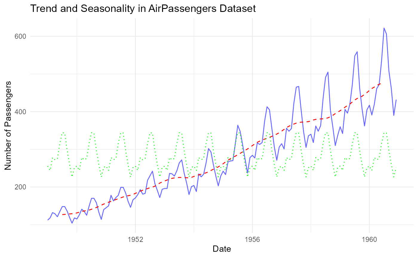
We can extract the trend and seasonality components from the decomposed time series.

# Decompose the time series
decomposed_ap <- decompose(AirPassengers_ts)

# Extract trend and seasonality
trend <- decomposed_ap$trend
seasonal <- decomposed_ap$seasonal

# Create a data frame for ggplot2
decomposed_df <- data.frame(
  Month = time(AirPassengers_ts),
  Passengers = as.numeric(AirPassengers_ts),
  Trend = trend,
  Seasonal = seasonal
)

# Plot trend and seasonality
ggplot(decomposed_df, aes(x = Month)) +
  geom_line(aes(y = Passengers), color = "blue", alpha = 0.6) +
  geom_line(aes(y = Trend), color = "red", linetype = "dashed") +
  geom_line(aes(y = Seasonal + mean(Passengers)), color = "green", linetype = "dotted") +
  labs(title = "Trend and Seasonality in AirPassengers Dataset",
       x = "Date", y = "Number of Passengers") +
  theme_minimal()
#> Don't know how to automatically pick scale for object of type <ts>. Defaulting
#> to continuous.
#> Warning: Removed 12 rows containing missing values or values outside the scale range
#> (`geom_line()`).

Conclusion

The timeSeriesDataSets package provides a rich collection of time series datasets for analysis. With these datasets, you can perform various time series analyses and gain insights into trends and patterns over time. The timeSeriesDataSets package aims to provide a comprehensive set of time series datasets that have been sourced from various R packages and modified to fit specific time series object conventions. This package should be a valuable resource for anyone working with time series data in R.

We encourage you to explore the datasets and leverage the functionality of this package to enhance your time series analysis and research.